Classification Using a Biplane Convolutional Neural Network

import numpy as np

First we create 80 point clouds of a torus, a sphere, and a swiss role each. Each point cloud consists of 125 points from the surface and 125 points of random noise. From each point cloud we take 80 subsamples of 30 points each and save all of these sumbsamples in the NumPy array point_clouds. See here for the source code.

from create_point_clouds import create_point_clouds

point_clouds: np.ndarray = create_point_clouds(
    seed = 2_000,
    nb_point_clouds = 80,
    nb_coarsened = 50
)

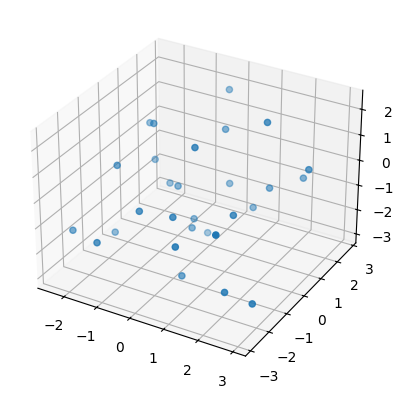
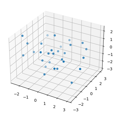
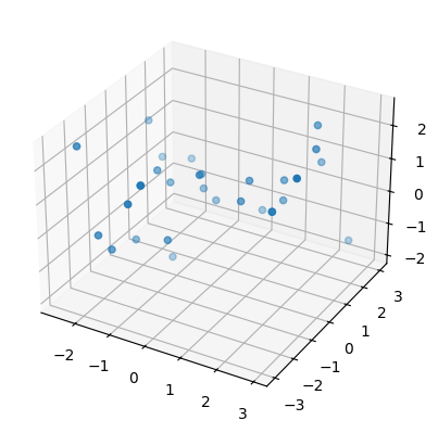
Then we plot one of these newly created point clouds (subsamples to be precise) for each surface.

from tadasets import plot3d

sphere, torus, swiss_roll = point_clouds[:,0,0]

plot3d( sphere     );
plot3d( torus      );
plot3d( swiss_roll );

Then we compute persistence intervals for each point cloud (subsamples to be precise).

from gudhi_util import (
    point_clouds_to_simplex_trees,
    simplex_trees_to_persistence_intervals_in_dim
)

simplex_trees = point_clouds_to_simplex_trees( point_clouds )

persistence_intervals = [
    np.arctan(
        simplex_trees_to_persistence_intervals_in_dim(
            simplex_trees = simplex_trees,
            dim = d
        )
    ) for
    d in range(3)
]

Then we merge all subsamples coming from the same point cloud and compute the corresponding biplanes.

import torch
torch.manual_seed( 3_000 )

from persunraveltorch.nn import BiplaneFromIntervals

#nb_coarsened = persistence_intervals[0].shape[2]

def to_torch_n_flatten_subsamples( array: np.ndarray ) -> torch.Tensor:
    return torch.from_numpy( np.float32(array) ).flatten(
        start_dim = 2,
        end_dim = 3
    )

pixel_columns = 36
padding = 4

biplane_from_intervals = BiplaneFromIntervals(
    pixel_columns = pixel_columns,
    padding = padding,
    max_overhead = 2**31
)

biplane = biplane_from_intervals(
    map(to_torch_n_flatten_subsamples, persistence_intervals)
) #/ nb_coarsened

Then we split the resulting biplanes into 60 biplanes for each surface for training and 20 biplanes for each surface for testing. We also normalize the biplanes and we initialize DataLoaders for training and testing.

from torch.utils.data import TensorDataset, DataLoader
from standard_scaler import StandardScaler

training_biplane, testing_biplane = biplane.split(60, dim=1)

labels = torch.Tensor([[0], [1], [2]]).long()

training_labels = labels.expand( *training_biplane.shape[:2] )
testing_labels  = labels.expand(  *testing_biplane.shape[:2] )

standard_scaler = StandardScaler( *torch.std_mean(training_biplane) )

training_dataset = TensorDataset(
    standard_scaler( training_biplane ).flatten(0, 1),
    #training_biplane.flatten(0, 1),
    training_labels.flatten(0, 1)
)
testing_dataset = TensorDataset(
    standard_scaler( testing_biplane ).flatten(0, 1),
    #testing_biplane.flatten(0, 1),
    testing_labels.flatten(0, 1)
)

batch_size = 30

training_dataloader = DataLoader(
    training_dataset,
    batch_size = batch_size,
    shuffle = True
)
testing_dataloader  = DataLoader(
    testing_dataset,
    batch_size = batch_size
)

Then we specify a biplane convolutional neural network and instantiate it with hyperparameters matching the present experiment.

import torch.nn as nn
import torch.nn.functional as F

from persunraveltorch.nn import (
    ConvBiplane,
    MaxPoolBiplane
)

class BiplaneCNN(nn.Module):
    
    def __init__(self,
                 *,
                 pixel_columns: int, # should be divisible by 2
                 padding_input: int,
                 top_dim: int,
                 nb_classes: int
                 ) -> None:

        super().__init__()

        kernel_size = (3, 3, 4)
        
        self.conv = nn.Sequential(
            ConvBiplane( 2, 4, kernel_size, shift = pixel_columns ),
            nn.ReLU(),
            MaxPoolBiplane(2),
            ConvBiplane( 4, 8, kernel_size, shift = pixel_columns // 2 ),
            nn.ReLU(),
            MaxPoolBiplane(2),
            nn.Flatten()
        )

        conv_out_features = self.conv(
            BiplaneFromIntervals(
                pixel_columns = pixel_columns,
                padding = padding_input# ,
                # device = 'meta'
            )( [torch.Tensor([]).view(0, 2)] * (top_dim + 1) ).unsqueeze(0)
        ).shape[1]

        self.final_layer = nn.Linear( conv_out_features, nb_classes )

    def forward(self,
                input: torch.Tensor
                ) -> torch.Tensor:
        return self.final_layer( self.conv(input) )

model = BiplaneCNN(
    pixel_columns = pixel_columns,
    padding_input = padding,
    top_dim = 2,
    nb_classes = 3
)

#initial_first_filters = model.state_dict()['conv.0.conv3d.weight'].clone().detach()

Then we run through 151 epochs of training and testing.

from train_test import (
    ProcessBatch,
    Optimize,
    accumulate_loss,
    accumulate_score
)

loss_fn = torch.nn.CrossEntropyLoss()

process_batch = ProcessBatch( model = model, loss_fn = loss_fn )

optimize = Optimize( torch.optim.Adam(model.parameters(), lr=0.003) )

epochs = 151

for t in range(epochs):
    model.train()
    training_results = [
        optimize(process_batch(*batch)) for batch in training_dataloader
    ]
    if t % 10 == 0:
        print(f"Epoch {t+1}\n-------------------------------")
        print(
            f"Training cross entropy: {accumulate_loss(training_results):>8f}"
        )
        model.eval()
        with torch.no_grad():
            testing_results = [
                process_batch(*batch) for batch in testing_dataloader
            ]
        print(f"Testing cross entropy: {accumulate_loss(testing_results):>8f}")
        accuracy = (
            accumulate_score( testing_results ) /
            len( testing_dataloader.dataset )
        )
        print(f"Testing accuracy: {100 * accuracy:>0.1f}%\n")

Epoch 1
-------------------------------
Training cross entropy: 1.392518
Testing cross entropy: 1.161076
Testing accuracy: 65.0%

Epoch 11
-------------------------------
Training cross entropy: 0.961834
Testing cross entropy: 0.883030
Testing accuracy: 90.0%

Epoch 21
-------------------------------
Training cross entropy: 0.266338
Testing cross entropy: 0.233634
Testing accuracy: 85.0%

Epoch 31
-------------------------------
Training cross entropy: 0.086513
Testing cross entropy: 0.038403
Testing accuracy: 100.0%

Epoch 41
-------------------------------
Training cross entropy: 0.042419
Testing cross entropy: 0.038774
Testing accuracy: 100.0%

Epoch 51
-------------------------------
Training cross entropy: 0.024842
Testing cross entropy: 0.015276
Testing accuracy: 100.0%

Epoch 61
-------------------------------
Training cross entropy: 0.013507
Testing cross entropy: 0.007967
Testing accuracy: 100.0%

Epoch 71
-------------------------------
Training cross entropy: 0.017682
Testing cross entropy: 0.009180
Testing accuracy: 100.0%

Epoch 81
-------------------------------
Training cross entropy: 0.004693
Testing cross entropy: 0.003792
Testing accuracy: 100.0%

Epoch 91
-------------------------------
Training cross entropy: 0.033343
Testing cross entropy: 0.010330
Testing accuracy: 100.0%

Epoch 101
-------------------------------
Training cross entropy: 0.022077
Testing cross entropy: 0.003151
Testing accuracy: 100.0%

Epoch 111
-------------------------------
Training cross entropy: 0.002178
Testing cross entropy: 0.001736
Testing accuracy: 100.0%

Epoch 121
-------------------------------
Training cross entropy: 0.001464
Testing cross entropy: 0.001573
Testing accuracy: 100.0%

Epoch 131
-------------------------------
Training cross entropy: 0.001168
Testing cross entropy: 0.001780
Testing accuracy: 100.0%

Epoch 141
-------------------------------
Training cross entropy: 0.000975
Testing cross entropy: 0.001475
Testing accuracy: 100.0%

Epoch 151
-------------------------------
Training cross entropy: 0.000853
Testing cross entropy: 0.001478
Testing accuracy: 100.0%

#torch.save(model.state_dict(), './successful-run.pt')

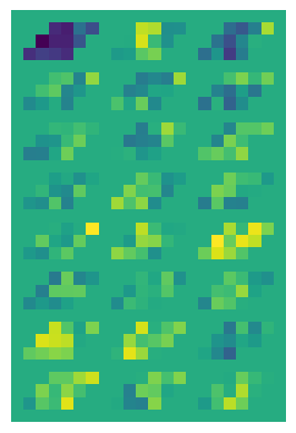
Finally we plot the filters of the first biplane convolutional layer. Each row corresponds to a pair of an input and an output channel. The top four rows correspond to the Hilbert function of the unravelled relative homology lattice as an input channel and four rows at the bottom to the unravelled rank invariant as an input channel.

import matplotlib.pyplot as plt
from persunraveltorch.nn import Reshear

first_filters, _ = Reshear.create_n_apply(
    model.state_dict()['conv.0.conv3d.weight'].clone().detach()
)

first_filters_unravelled = F.pad(
    pad = (1, 0, 1, 0),
    input = F.pad(
        pad = (0, 1, 0, 1),
        input = first_filters
    ).swapaxes(2, 3).swapaxes(0, 1).flatten(
        start_dim=3,
        end_dim=4
    ).flatten(end_dim=2)
)

_, ax = plt.subplots()

ax.matshow( first_filters_unravelled.numpy() )
ax.axis( 'off' );