Binary Classification Using an SVM and Subsequent Regularization
from typing import Tuple

import numpy as np
First we create 40 point clouds of a torus and a sphere each.
Each point cloud consists of 125 points from the surface
and 125 points of random noise.
From each point cloud we take 25 subsamples of 30 points each
and save all of these sumbsamples in the NumPy array point_clouds.
See
here for the source code.
from create_point_clouds import create_point_clouds

point_clouds = create_point_clouds(
    nb_point_clouds = 40,
    nb_coarsened = 25
)[:2]
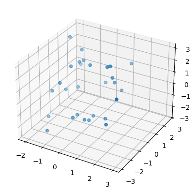
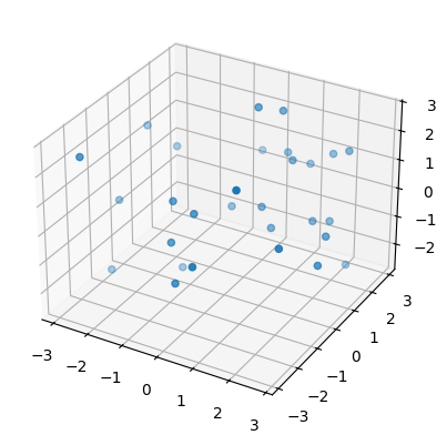
Then we plot one of these newly created point clouds (subsamples to be precise) for each surface.
from tadasets import plot3d

sphere, torus = point_clouds[:,0,0]

plot3d( sphere );
plot3d( torus  );


Then we compute persistence intervals for each point cloud (subsamples to be precise).
from gudhi_util import (
    point_clouds_to_simplex_trees,
    simplex_trees_to_persistence_intervals_in_dim
)

simplex_trees = point_clouds_to_simplex_trees( point_clouds )

persistence_intervals = [
    simplex_trees_to_persistence_intervals_in_dim(
        simplex_trees = simplex_trees,
        dim = d
    ) for
    d in range(3)
]
Then we merge all subsamples (persistence intervals thereof) coming from the same point cloud and we split the result into 10 point clouds (persistence intervals thereof) from each surface for training and 30 point clouds from each surface for testing.
import torch

nb_coarsened = persistence_intervals[0].shape[2]

def preprocess_n_split(array: np.ndarray
                       ) -> Tuple[torch.Tensor, torch.Tensor]:
    return torch.from_numpy( np.float32(np.arctan(array)) ).flatten(
        start_dim = 2,
        end_dim = 3
    ).split( (10, 30), dim = 1 )

training_dgms, testing_dgms = zip(
    *map( preprocess_n_split, persistence_intervals )
)
Then we create matching labels for training and testing.
labels = torch.Tensor( [[0], [1]] )

training_labels = labels.expand( *training_dgms[0].shape[:2] ).flatten(0, 1)
testing_labels  = labels.expand(  *testing_dgms[0].shape[:2] ).flatten(0, 1)

training_dgms_flat = [ dgm.flatten(0, 1) for dgm in training_dgms ]
testing_dgms_flat  = [ dgm.flatten(0, 1) for dgm in  testing_dgms ]
Then we compute the Gram matrix with respect to the inner product of Hilbert functions of the associated unravelled relative homology lattices for the training data.
from persunraveltorch.nn import HilbertGram

hilbert_gram = HilbertGram()

# Here we could set
# training_gram = hilbert_gram(training_dgms_flat, training_dgms_flat)
# However, as this would allocate a large amount of RAM at once,
# we compute the Gram matrix one row at a time instead.
training_gram = torch.cat(
    [ hilbert_gram(dgm, training_dgms_flat) for
      dgm in
      zip(*training_dgms_flat)
     ]
).numpy() / nb_coarsened**2
Then we instantiate a support vector classifier and train it with the previously computed Gram matrix.
from scipy.special import expit
from sklearn import svm, metrics

clf = svm.SVC( kernel = 'precomputed' )

clf.fit( training_gram, training_labels.numpy() )
SVC(kernel='precomputed')In a Jupyter environment, please rerun this cell to show the HTML representation or trust the notebook.
On GitHub, the HTML representation is unable to render, please try loading this page with nbviewer.org.
Parameters
| C | 1.0 | |
| kernel | 'precomputed' | |
| degree | 3 | |
| gamma | 'scale' | |
| coef0 | 0.0 | |
| shrinking | True | |
| probability | False | |
| tol | 0.001 | |
| cache_size | 200 | |
| class_weight | None | |
| verbose | False | |
| max_iter | -1 | |
| decision_function_shape | 'ovr' | |
| break_ties | False | |
| random_state | None |
Then we compute the Gram matrix for testing and we test the previously trained support vector classifier.
from gram_test import GramTest

support_indices = torch.from_numpy( np.int64(clf.support_) )

gram_test = GramTest(
    gram = hilbert_gram,
    support_indices = support_indices,
    len_train = len( training_dgms_flat[0] ),
    support_vectors = [
        intervals[support_indices] for
        intervals in
        training_dgms_flat
    ]
)

testing_gram = torch.cat(
    [ gram_test(dgm) for dgm in zip(*testing_dgms_flat) ]
).numpy() / nb_coarsened**2

print(f"Model accuracy: {100 * metrics.accuracy_score(testing_labels.numpy(), clf.predict(testing_gram)):>0.1f}%")
print(f"Testing cross entropy: {metrics.log_loss(testing_labels.numpy(), expit(clf.decision_function(testing_gram))):.4f}")
print(f"Training cross entropy: {metrics.log_loss(training_labels.numpy(), expit(clf.decision_function(training_gram))):.4f}")
Model accuracy: 95.0%
Testing cross entropy: 0.2999
Training cross entropy: 0.2761
The we render a 2D bitmap corresponding to the normal of the affine hyperplane determined by our support vector classifier.
from persunraveltorch.nn import BiplaneFromIntervals

pixel_columns = 200
padding = 4

biplane_from_intervals = BiplaneFromIntervals(
    pixel_columns = pixel_columns,
    padding = padding,
    max_overhead = 2**31
)

training_bitmap = (
    biplane_from_intervals( training_dgms_flat )[:,0,0] / nb_coarsened
)
normal = torch.einsum(
    'ij,jkl->kl',
    torch.from_numpy( np.float32(clf.dual_coef_) ),
    training_bitmap[clf.support_]
)

testing_bitmap = (
    biplane_from_intervals( testing_dgms_flat )[:,0,0] / nb_coarsened
)
Then we describe the decision function of the support vector classifier as a decision function on 2D bitmaps thought of as Hilbert functions and we test whether we get approximately the same accuracy and cross entropy as with the support vector classifier.
import torch.nn as nn
import torch.nn.functional as F
from persunraveltorch.nn import StripAffineFunctional

strip_affine_functional = StripAffineFunctional(
    weight = normal.clone().detach(),
    bias = torch.tensor( clf.intercept_[0] ),
    pixel_area = biplane_from_intervals.pixel_area
)

model = nn.Sequential(
    strip_affine_functional,
    nn.Sigmoid()
)

model.eval()

with torch.no_grad():
    pred = model(testing_bitmap)
    print( f"Reconstructed model accuracy: {100 * pred.round().eq(testing_labels).float().mean():0.1f}%" )
    print( f"Reconstructed testing cross entropy: {F.binary_cross_entropy(pred, testing_labels):0.4f}" )
Reconstructed model accuracy: 95.0%
Reconstructed testing cross entropy: 0.2963
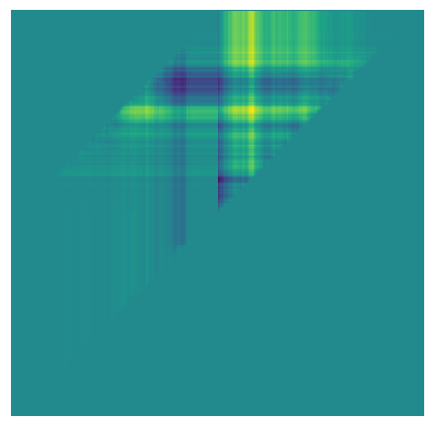
Then we plot the normal we computed as a pseudocolor image.
import matplotlib.pyplot as plt
from persunraveltorch.nn import Reshear, ReshearMode

reshear = Reshear(shape = normal.shape, mode = ReshearMode.ZERO)

def viz_normal():
    _, ax = plt.subplots( figsize = (7.2, 4.8) )

    ax.axis('off')
    ax.matshow(
        reshear(
            strip_affine_functional.weight.detach()
        ).numpy()[:,pixel_columns:]
    )
    #_, axs = plt.subplots( ncols = 2 )

    #axs[0].axis('off')
    #axs[1].axis('off')
    #axs[0].matshow(           normal.numpy() )
    #axs[1].matshow( resheared_normal.numpy() )

viz_normal()

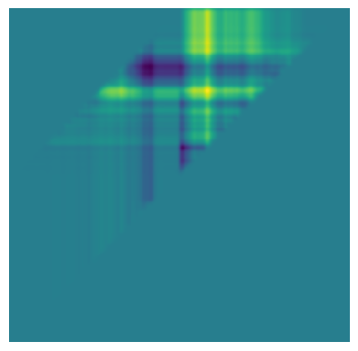
As the previous plot shows a large degree of variation, we try to regularize it using logistic regression with penalties for the normal and its gradient. We note however, that in order to obtain the effect seen here, we have to make the penalties so large, that the cross entropy is of little influence in the optimization. So really, the following logistic regression is no more than a fancy way of blurring an image and shown here merely to explore the design space.
optimizer = torch.optim.SGD( model.parameters(), lr = 0.9 )

epochs = 100

for t in range(epochs):
    model.train()
    penalty = strip_affine_functional.energy()
    variational_penalty = strip_affine_functional.variational_energy() / 100
    cross_entropy = F.binary_cross_entropy(
        model(training_bitmap),
        training_labels
    )
    loss = variational_penalty + penalty + cross_entropy
    loss.backward()
    optimizer.step()
    optimizer.zero_grad()
    model.eval()
    if t % 10 == 0:
        print(f"Epoch {t+1}\n-------------------------------")
        print( f"Cross entropy: {cross_entropy:0.8f}" )
        print( f"Penalty: {penalty:0.4f}" )
        print( f"Variational penalty: {variational_penalty:0.4f}" )
        with torch.no_grad():
            pred = model( testing_bitmap )
            print( f"Testing cross entropy: {F.binary_cross_entropy(pred, testing_labels):0.8f}" )
            print( f"Testing accuracy: {100 * pred.round().eq(testing_labels).float().mean():0.1f}%\n" )
Epoch 1
-------------------------------
Cross entropy: 0.27560246
Penalty: 7.0315
Variational penalty: 76.4522
Testing cross entropy: 0.29659453
Testing accuracy: 95.0%

Epoch 11
-------------------------------
Cross entropy: 0.27745908
Penalty: 6.8860
Variational penalty: 44.3300
Testing cross entropy: 0.29858875
Testing accuracy: 95.0%

Epoch 21
-------------------------------
Cross entropy: 0.27903256
Penalty: 6.7884
Variational penalty: 31.2262
Testing cross entropy: 0.29987636
Testing accuracy: 95.0%
Epoch 31
-------------------------------
Cross entropy: 0.28036216
Penalty: 6.7118
Variational penalty: 24.8344
Testing cross entropy: 0.30084115
Testing accuracy: 95.0%

Epoch 41
-------------------------------
Cross entropy: 0.28152493
Penalty: 6.6463
Variational penalty: 21.1729
Testing cross entropy: 0.30163822
Testing accuracy: 95.0%

Epoch 51
-------------------------------
Cross entropy: 0.28257304
Penalty: 6.5876
Variational penalty: 18.7969
Testing cross entropy: 0.30233893
Testing accuracy: 95.0%
Epoch 61
-------------------------------
Cross entropy: 0.28353912
Penalty: 6.5334
Variational penalty: 17.1106
Testing cross entropy: 0.30297989
Testing accuracy: 95.0%

Epoch 71
-------------------------------
Cross entropy: 0.28444493
Penalty: 6.4827
Variational penalty: 15.8348
Testing cross entropy: 0.30358166
Testing accuracy: 95.0%

Epoch 81
-------------------------------
Cross entropy: 0.28530440
Penalty: 6.4346
Variational penalty: 14.8235
Testing cross entropy: 0.30415609
Testing accuracy: 95.0%
Epoch 91
-------------------------------
Cross entropy: 0.28612703
Penalty: 6.3887
Variational penalty: 13.9934
Testing cross entropy: 0.30471048
Testing accuracy: 95.0%
viz_normal();
